Make Diffusion model from scratch ( easy way to implement quick diffusion model )

This article is a tutorial on building a diffusion model from scratch by yourself. ( using TensorFlow / also have a PyTorch version provided )

Published in

tree.rocks

7 min readApr 10, 2023

I always like to make things simple and easy. So in here we’re avoiding complicated math. This is not a normal diffusion model. Instead, I call this quick diffusion model. Will only use Convolutional Neural Network (CNN) to make diffusion model.

I won’t give you any existing model/weights/scripts files in this article.
You need to train your model by yourself.
( We are using the CIFAR-10 dataset provided by TensorFlow. )

You can find code in my GitHub ( Tensorflow version )
https://github.com/Seachaos/Tree.Rocks/blob/main/QuickDiffusionModel/QuickDiffusionModel.ipynb

If you are looking for the PyTorch version, you can find it here:
https://github.com/Seachaos/Tree.Rocks/blob/main/QuickDiffusionModel/QuickDiffusionModel_torch.ipynb

The Idea

This is how the diffusion model works: it’s like based with a fully noisy image and gradually improves the image quality until it becomes clear.
( As below image showed )

the example of diffusion model improves the image

Therefore, we can create a Deep Learning model that can improve image quality ( from fully noise to clear image ), the flow idea:

For a clearer idea, take a look at this additional flow chart.

how the image flow in the diffusion model

As you can see in the image above, the model is attempting to produce an image with progressively less noise.

Now, we just need to train a Deep Learning model to learn how to reduce noise.
For that mission, we need two input in our model:

input image — the noise image need to be processed
timestamp — tell model what’s noise status so can be easier to learn

Implement Quick Diffusion Model

First thing first, let’s import what we needed:

import numpy as np

from tqdm.auto import trange, tqdm
import matplotlib.pyplot as plt

import tensorflow as tf
from tensorflow.keras import layers

and prepare our datasets, In this tutorial, we will be using a lot of car images ( CIFAR-10 ) for examples to make things as simple and quick as possible.
( However, if you have enough samples, you can choose any image you prefer. )

(X_train, y_train), (X_test, y_test) = tf.keras.datasets.cifar10.load_data()
X_train = X_train[y_train.squeeze() == 1]
X_train = (X_train / 127.5) - 1.0

Next, let’s define the variables.

IMG_SIZE = 32     # input image size, CIFAR-10 is 32x32
BATCH_SIZE = 128  # for training batch size
timesteps = 16    # how many steps for a noisy image into clear
time_bar = 1 - np.linspace(0, 1.0, timesteps + 1) # linspace for timesteps

Here, we set “timesteps”, This means that our model will learn to produce images from noisy (level 0) to clear (level 16) through the training process.

Let’s see an image for more clear idea

plt.plot(time_bar, label='Noise')
plt.plot(1 - time_bar, label='Clarity')
plt.legend()

the image noise and clarity with time step

As you can see, from time step 0 to 16, the noise is reduced and clarity is progressively improving. that’s what we want our model to learn.

And prepare some function for preview data

def cvtImg(img):
    img = img - img.min()
    img = (img / img.max())
    return img.astype(np.float32)

def show_examples(x):
    plt.figure(figsize=(10, 10))
    for i in range(25):
        plt.subplot(5, 5, i+1)
        img = cvtImg(x[i])
        plt.imshow(img)
        plt.axis('off')

show_examples(X_train)

Training Prepare

In here, we need the code for prepare training images.

The idea is to obtain two images (A and B) from random time points, , where A is a noisy image and B is a much clearer image.
Our model will learn to transform A into B (from noisy to clearer) based on that specific time point.
( as this image again )

Therefore, we have forward_noise function here.

def forward_noise(x, t):
    a = time_bar[t]      # base on t
    b = time_bar[t + 1]  # image for t + 1
    
    noise = np.random.normal(size=x.shape)  # noise mask
    a = a.reshape((-1, 1, 1, 1))
    b = b.reshape((-1, 1, 1, 1))
    img_a = x * (1 - a) + noise * a
    img_b = x * (1 - b) + noise * b
    return img_a, img_b
    
def generate_ts(num):
    return np.random.randint(0, timesteps, size=num)

# t = np.full((25,), timesteps - 1) # if you want see clarity
# t = np.full((25,), 0)             # if you want see noisy
t = generate_ts(25)             # random for training data
a, b = forward_noise(X_train[:25], t)
show_examples(a)

If you want to understand how it works, I recommend running the code that I have commented out. ( t = … )

Build CNN Block

We will use U-Net for our model
The details will be explained in the code that follows.

Model architecture, the details will be explained in the code that follows

Before we can build the model, we need to define the blocks first.
Here is the code for make block:

def block(x_img, x_ts):
    x_parameter = layers.Conv2D(128, kernel_size=3, padding='same')(x_img)
    x_parameter = layers.Activation('relu')(x_parameter)

    time_parameter = layers.Dense(128)(x_ts)
    time_parameter = layers.Activation('relu')(time_parameter)
    time_parameter = layers.Reshape((1, 1, 128))(time_parameter)
    x_parameter = x_parameter * time_parameter
    
    # -----
    x_out = layers.Conv2D(128, kernel_size=3, padding='same')(x_img)
    x_out = x_out + x_parameter
    x_out = layers.LayerNormalization()(x_out)
    x_out = layers.Activation('relu')(x_out)
    
    return x_out

Each block contains two convolutional networks with a time parameter, allowing the network to determine its current time step and output corresponding information.
You can see block flow chart:
( x_img is input image which is noisy image, x_ts is input for time step )

Build Model

Now we can build our model

def make_model():
    x = x_input = layers.Input(shape=(IMG_SIZE, IMG_SIZE, 3), name='x_input')
    
    x_ts = x_ts_input = layers.Input(shape=(1,), name='x_ts_input')
    x_ts = layers.Dense(192)(x_ts)
    x_ts = layers.LayerNormalization()(x_ts)
    x_ts = layers.Activation('relu')(x_ts)
    
    # ----- left ( down ) -----
    x = x32 = block(x, x_ts)
    x = layers.MaxPool2D(2)(x)
    
    x = x16 = block(x, x_ts)
    x = layers.MaxPool2D(2)(x)
    
    x = x8 = block(x, x_ts)
    x = layers.MaxPool2D(2)(x)
    
    x = x4 = block(x, x_ts)
    
    # ----- MLP -----
    x = layers.Flatten()(x)
    x = layers.Concatenate()([x, x_ts])
    x = layers.Dense(128)(x)
    x = layers.LayerNormalization()(x)
    x = layers.Activation('relu')(x)

    x = layers.Dense(4 * 4 * 32)(x)
    x = layers.LayerNormalization()(x)
    x = layers.Activation('relu')(x)
    x = layers.Reshape((4, 4, 32))(x)
    
    # ----- right ( up ) -----
    x = layers.Concatenate()([x, x4])
    x = block(x, x_ts)
    x = layers.UpSampling2D(2)(x)
    
    x = layers.Concatenate()([x, x8])
    x = block(x, x_ts)
    x = layers.UpSampling2D(2)(x)
    
    x = layers.Concatenate()([x, x16])
    x = block(x, x_ts)
    x = layers.UpSampling2D(2)(x)
    
    x = layers.Concatenate()([x, x32])
    x = block(x, x_ts)
    
    # ----- output -----
    x = layers.Conv2D(3, kernel_size=1, padding='same')(x)
    model = tf.keras.models.Model([x_input, x_ts_input], x)
    return model

model = make_model()
# model.summary()

This is a U-Net, and the left, right, and MLP parts can be referenced in the image above (Model architecture).

Don’t forget compile model

optimizer = tf.keras.optimizers.Adam(learning_rate=0.0008)
loss_func = tf.keras.losses.MeanAbsoluteError()
model.compile(loss=loss_func, optimizer=optimizer)

We using Adam for optimizer and MeanAbsoluteError ( MAE ) for loss function.

Predict the result

We can now try our first prediction. The steps for prediction are as follows:

create noisy images
input to our model with time step
keep doing this until end of time step

So here is this function:

def predict(x_idx=None):
    x = np.random.normal(size=(32, IMG_SIZE, IMG_SIZE, 3))
    for i in trange(timesteps):
        t = i
        x = model.predict([x, np.full((32), t)], verbose=0)
    show_examples(x)

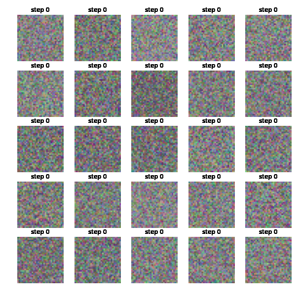
predict()

Above is our Non-Trained Model output, as you can see, it’s nothing useful.

Also this function can help us see each steps:

def predict_step():
    xs = []
    x = np.random.normal(size=(8, IMG_SIZE, IMG_SIZE, 3))

    for i in trange(timesteps):
        t = i
        x = model.predict([x, np.full((8),  t)], verbose=0)
        if i % 2 == 0:
            xs.append(x[0])

    plt.figure(figsize=(20, 2))
    for i in range(len(xs)):
        plt.subplot(1, len(xs), i+1)
        plt.imshow(cvtImg(xs[i]))
        plt.title(f'{i}')
        plt.axis('off')

predict_step()

Training Model

This training function is simple

def train_one(x_img):
    x_ts = generate_ts(len(x_img))
    x_a, x_b = forward_noise(x_img, x_ts)
    loss = model.train_on_batch([x_a, x_ts], x_b)
    return loss

We simply need to provide x_ts and x_img (x_a) to enable our model to learn how to generate x_b. ( denoise image )

and make it as epoch function

def train(R=50):
    bar = trange(R)
    total = 100
    for i in bar:
        for j in range(total):
            x_img = X_train[np.random.randint(len(X_train), size=BATCH_SIZE)]
            loss = train_one(x_img)
            pg = (j / total) * 100
            if j % 5 == 0:
                bar.set_description(f'loss: {loss:.5f}, p: {pg:.2f}%')

finally, run it many times and gradually reduce learning rate

for _ in range(10):
    train()
    # reduce learning rate for next training
    model.optimizer.learning_rate = max(0.000001, model.optimizer.learning_rate * 0.9)

    # show result 
    predict()
    predict_step()
    plt.show()

You can get some output images like this

Conclusion

This tutorial is designed to be simple, allowing you to experiment. You can try your own parameters ( like change image size, CNN filters, time steps or MLP … ) and more epochs training to get better result.

Here are some examples of during the training model